Office 2007 has several new features but some precincts for old Office 2003 users who were familiar with the menu interface. The new ribbon interface of Excel is quite easy and provides almost all functions fight in the range of you r mouse click. To insert a Pie chart more effectively and give a professional look to your spreadsheet, follow these steps:
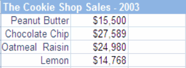
1. Enter the data:
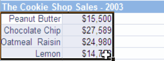
Remember, this the sample data. You can enter your own data accordingly. After entering the data you have to select the data
2. Select the Pie Chart from the Chart Type
Choose relevant Pie chart type in the pie chart list from the Insert ribbon. For example, I selected the Pie in 3-D and the result is as under:
3. Format the Pie Chart
By clicking on the chart, you can see a new ribbon “Chart Tools” which has three sub sections as shown in the figures below:
(Select color schemes and designs from here)
(Select title, legend position and data labels from here)
(Select text formatting, outline and fill options from here)


No comments:
Post a Comment